The Temporal Cave
Testing the Platonic Representation Hypothesis for video
In Plato’s Allegory of the Cave, prisoners observe only shadows on the wall and mistake them for reality — their perception is a projection of a deeper truth they cannot directly access. Machine learning models face a similar situation: they observe training data, which is only an incomplete picture of reality, and construct internal representations accordingly.
The Platonic Representation Hypothesis posits that as models grow larger and more capable, their internal representations converge onto a true underlying reality. It predicts that models trained on different architectures or with different objectives will eventually learn the same representation as data and capacity increase. This project tests that hypothesis in the video domain: do contrastive learners and autoencoders trained on the same video data converge to similar representations, and how does the temporal window Δt affect that convergence?
Datasets. We run experiments on two datasets with different visual complexity:
- Moving MNIST — 10,000 sequences of 20 frames at 64×64. Two digits moving across a black background; controlled, computationally tractable.
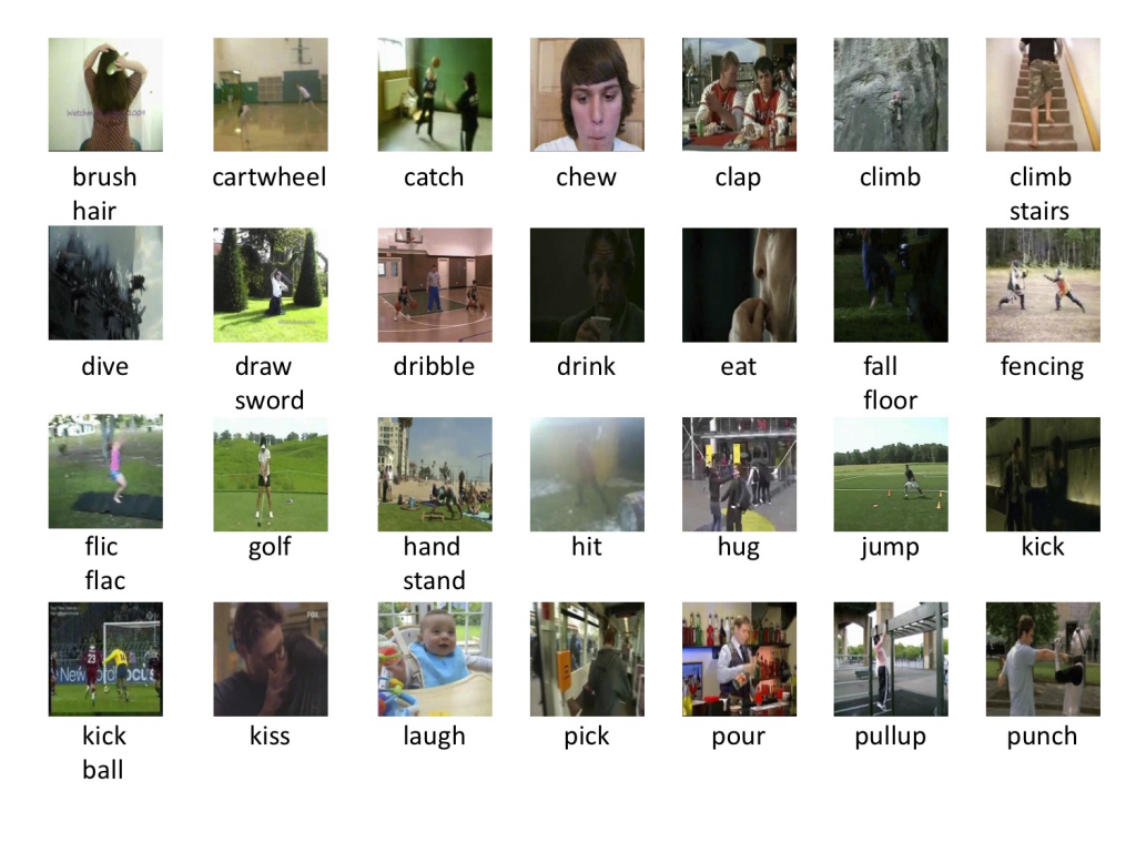
- HMDB51 — ~7,000 clips across 51 action classes (brush hair, cartwheel, dive, fencing…). More naturalistic and visually complex.
Methods. We train a contrastive learner using temporally-close frames as positive pairs — frames within Δt seconds are treated as views of the same underlying scene state, all other frames as negatives. We train an autoencoder on the same data using MSE reconstruction loss, with no temporal signal at all. Both share the same convolutional encoder architecture producing a 256-dimensional latent space. To compare them we use a mutual k-nearest-neighbor metric: for each frame, we find its k nearest neighbors in both latent spaces and measure the overlap.
The diagram below shows the full training setup and where the temporal window Δt enters it.
Figure: two objectives, one encoder — the contrastive branch treats frames within Δt as views of the same scene state, while the autoencoder sees each frame in isolation; both map into a 256-d latent space.
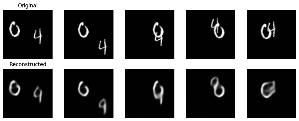
Results — autoencoder reconstruction. The autoencoder reconstructs Moving MNIST frames as blurred versions of the originals, capturing the main digit structure even when individual digits are not perfectly sharp.
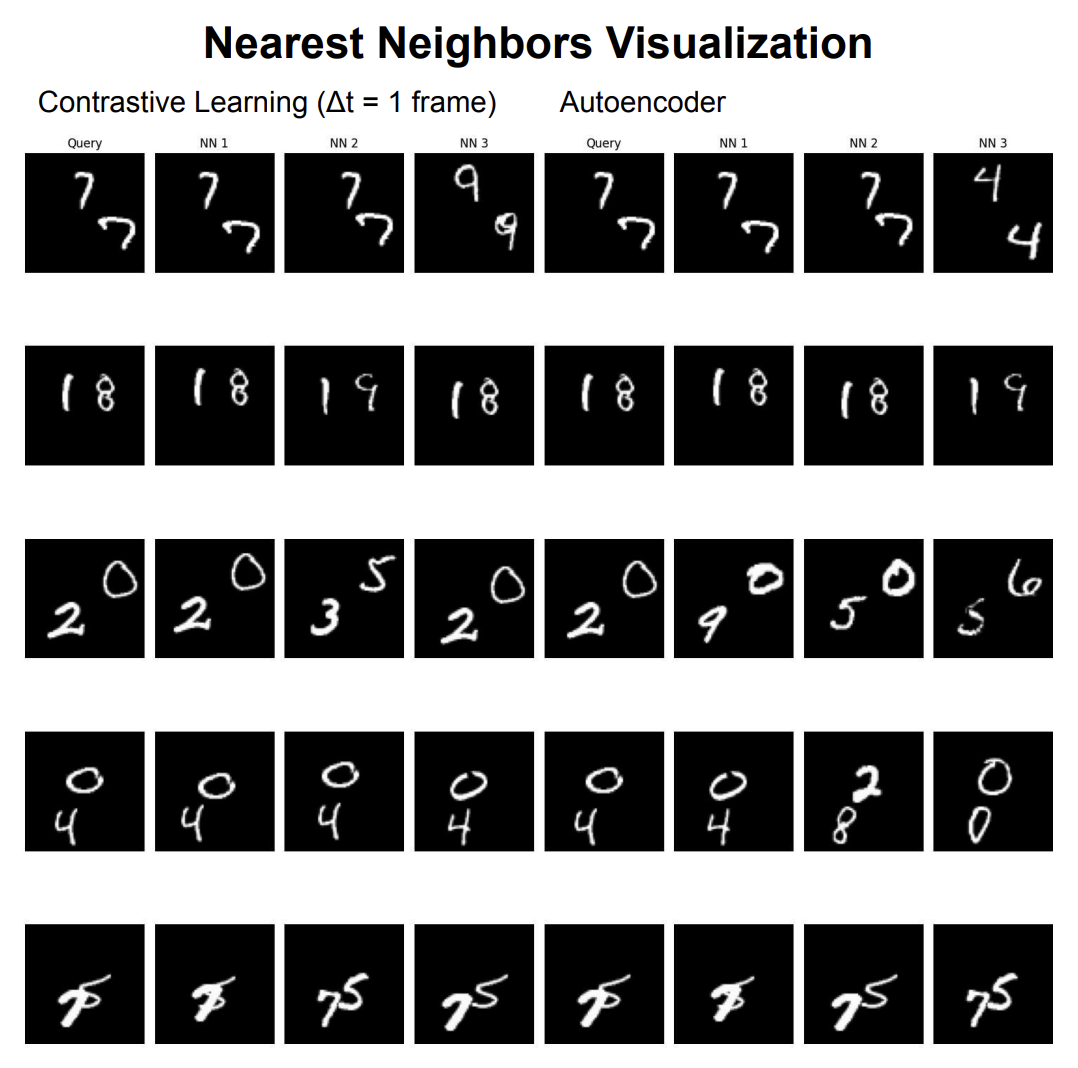
Results — nearest neighbor structure. At Δt=1 frame, contrastive learning forces the model to distinguish frames that are almost identical except for slight digit movement. The nearest neighbors it recovers look very similar to the query both in digit identity and position. The autoencoder’s neighbors track digit identity more loosely.
The diagram below shows how the mutual k-NN score used in the next experiment is computed.
Figure: the mutual k-NN metric — a query frame's k nearest neighbors are retrieved in each latent space, and similarity is the fraction of neighbors shared by both spaces (green).
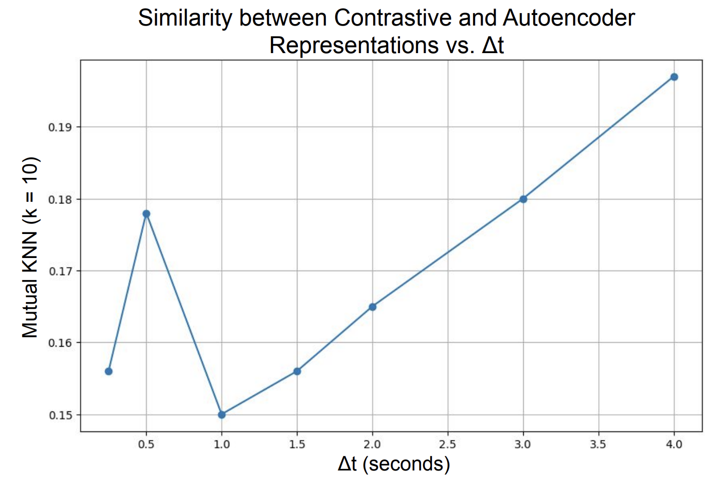
Results — similarity vs Δt. The key experiment: how does mutual KNN similarity between the two representations change as we vary Δt?
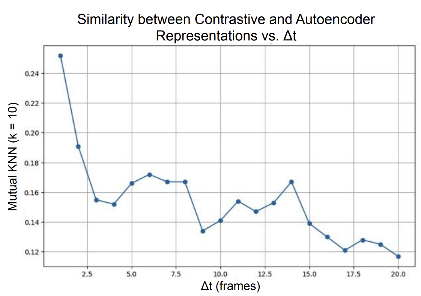
On Moving MNIST, similarity is highest at Δt=1 and decreases as Δt grows. Small temporal windows force contrastive representations to be very fine-grained and position-sensitive — close to what the autoencoder independently learns from pixel reconstruction. Larger windows push the contrastive model toward more abstract, temporally-invariant features that diverge from the autoencoder’s focus.
On HMDB51, the trend reverses: similarity increases with larger Δt. For complex naturalistic video, a wider temporal window pushes the contrastive learner toward semantic scene representations that better align with what the autoencoder recovers from the richer visual signal. This supports the Platonic Representation Hypothesis: in a sufficiently complex domain, representations from different objectives do converge.
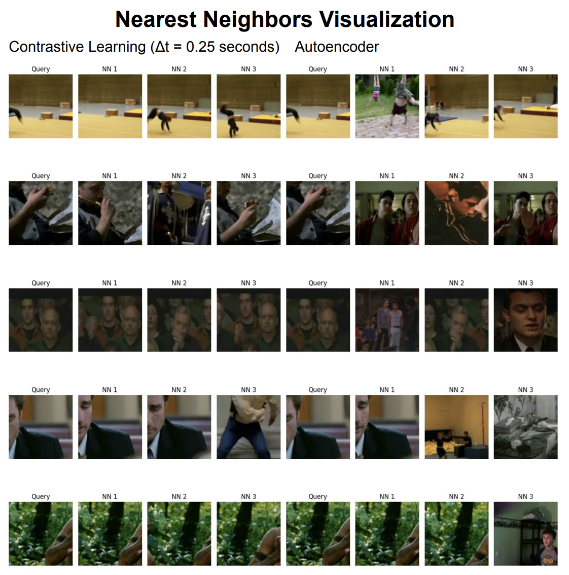
The two datasets tell complementary stories. In simple visual worlds, tight temporal supervision produces representations that match reconstruction-based ones at small Δt but diverge at large Δt. In complex visual worlds, wider temporal windows are needed to reach the level of abstraction where the two objectives converge. Whether this convergence continues toward a single true Platonic representation at larger scales remains an open question.
The sketch below summarizes the mechanism behind the two opposite trends.
Figure: why the two datasets trend in opposite directions — widening Δt pushes contrastive features from fine-grained toward abstract, and each dataset's autoencoder sits at a different point on that spectrum.
Final project for 6.7960 (Deep Learning), MIT. Joint work with Adithya Balachandran and Alex Gu.